


|
|
||||||||||||||||
|
|
|
|
|
|
|
|
|
|
|
|
|
|
|
|
|
|
|
|
|
|
|
|
|
|
|
|||||||||
|
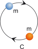
The Apparent Mystery of the Electron: There is no mystery! The electron can be physically understood! Since the middle of the 1920s physicists have been struggling to understand the electron. From experiments it was concluded that the electron is a structureless, point-like object, whose entire mass is concentrated in its extensionless centre. On the other hand the electron displays properties which normally result from an extended structure, namely angular momentum (spin), a magnetic moment, and some sort of an internal oscillation. In 1928, when Paul Dirac presented the wave function of the electron (the “Dirac equation”), it became obvious that there must be not only an internal oscillation but also some internal motion at the speed of light. When Erwin Schrödinger found this as a consequence of the Dirac equation, he gave the phenomenon the German name “Zitterbewegung”, which means some sort of poorly defined oscillation. Subsequently physicists attributed this intrinsic contradiction between the electron’s different properties to the common-sense view that the electron is subject to quantum mechanics and as such not accessible to the human imagination. However, a solution does exist, whose understanding relies on the application of the classical laws of physics and which is free of contradictions: if the electron is assumed to be made up of two massless constituent particles, then this assumption correctly predicts the experimental results. It provides the correct relationship between the parameters of the electron: its mass, its constant angular momentum (spin), and its magnetic moment. The assumption made above has been generalised for all elementary particles as a physical model called the "Basic Particle Model". (Note: This site is also available as a pdf file.) 1 Introduction The way to understand the electron classically is to accept that the electron has an extension, as assumed by the Basic Particle Model, and is not point-like, as stated by quantum mechanics. According to the Basic Particle Model every elementary particle is made up of 2 massless constituent particles, which orbit each other at the speed of light c. Their orbital frequency is the de Broglie frequency (Figure 1.1). The mass of the entire particle follows from the fact that it has extension. |
||||||||||||||||||
Figure 1.1: Structure
of an elementary Particle |
|||||||||||||||||||
|
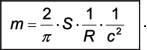
2 General Particle Properties 2.1 The Mass of the Electron The mass of the electron follows from the general fact that every extended object necessarily displays inertial behaviour. This is the mass mechanism of elementary particles. Due to this mechanism, the mass m of an elementary particle is generally described by the equation |
|||||||||||||||||||
|
|
(2.1) |
||||||||||||||||||
|
where ħ
is the reduced Planck constant, c the speed of light and R
the radius of the particle.
The
above formula (2.1) is valid for all elementary particles if their
electric charge is neglected. However, as the electron does have an
electric charge, the result given by (2.1) has to be refined by adding a
small correction factor (present in the Landé factor). This correction
is calculated in Appendix B. In the following we will refer to the general deduction of the particle properties, particularly the mass as given in the origin of mass. In addition to that deduction, this site will in particular deal with the properties of the electron that are caused by the presence of an electric charge. 2.2 The Magnetic Moment 2.2.1 The Basic Calculation
The
assumption of an extended electron helps us to understand the magnetic
moment using a classical view.
|
|||||||||||||||||||
|
|
(2.2) |
||||||||||||||||||
|
The current i flowing in a particle having one elementary charge e0 moving at speed c is simply: |
|||||||||||||||||||
|
|
(2.3) |
||||||||||||||||||
| with ν being the orbital frequency within the particle. Combining equations (2.2) and (2.3) we get: |
|
||||||||||||||||||
|
|
(2.4) | ||||||||||||||||||
| If R is now inserted from the mass formula (2.1), the magnetic moment turns out to be | |||||||||||||||||||
|
|
(2.5) | ||||||||||||||||||
|
For the electron this is the 'Bohr Magneton'. Remark: Please note that this important equation has been deduced here by classical means. Historically, some attempts to deduce the magnetic moment of the electron by classical means were made in the first half of the 20th century. These attempted deductions exclusively used the electromagnetic energy within the electron in order to find a relationship between its magnetic moment and its mass. The result of this calculation was wrong by a factor of typically >300. Later the correct relationship was provided by the Dirac equation of the electron. From this success it was concluded that the electron can be correctly understood and described only through quantum mechanics. - The success of the above classical deduction follows from the assumption that the force within the particle is primarily the strong force.
Eq. (2.1) can be used to calculate the size of the electron numerically. If the parameters |
|||||||||||||||||||
| me = 9.11 · 10 -31 kg for the mass of the electron | |||||||||||||||||||
| c = 2.988 · 108 m/s | |||||||||||||||||||
| ħ = 1.0546 · 10-34 m · kg / s2 | |||||||||||||||||||
|
are inserted in eq. (2.1), the result for the electron is |
|||||||||||||||||||
| Rei = 3.86 · 10-13 m. |
|
||||||||||||||||||
|
This is an unfamiliar result because the literature states that
experiments rule out any extension of this magnitude. However this
apparent conflict does not in fact exist, as is explained below.
Remark: If the mass of the electron is inserted in eq. (2.5), it yields the correct magnetic moment of the Bohr magneton |
|||||||||||||||||||
|
|
(2.6) |
||||||||||||||||||
|
results
from it. 2.2.2 The Correction for the Electric Influence As mentioned above, the magnetic moment of the electron is not exactly equal to the Bohr magneton but slightly greater, by a factor of approx. 10-3. Conventional physics (QED) attributes this difference to vacuum polarization effects around the electron. However, if the electric charge of the electron is taken into account, the radius of the electron is slightly larger than that caused by the strong force. The reason for this is presented in detail in Appendix B. - When this correction is used in the above calculation, we arrive at a similar correction to that performed by Julian Schwinger in 1948 using “vacuum polarization” [2]. It may be conjectured that any use of “vacuum polarization” or virtual particles is unnecessary if the Basic Particle Model is used; the Landé factor can be derived without resorting to quantum mechanics.
Equation (2.2) can be rearranged to give |
|||||||||||||||||||
|
|
(2.7) |
||||||||||||||||||
|
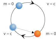
The left side is the formal definition of the angular momentum for v = c. The right side fulfils the expectation towards the spin of an elementary particle in so far as it is independent of any specific properties of the particle; so that its value is universal. The factor 1 on the right side however is unsatisfactory at first glance as the measured spin corresponds to a factor of ½. It should, however, not come as a surprise. Eq. (2.7) would represent the angular momentum of two objects orbiting each other, where each carries half of the classical mass of an electron. The configuration of the Basic Particle Model is, however, different in that the two objects (basic particles) do not have any classical mass. In addition, the field which enforces the continuous motion of the basic particles does not act on the basic particles tangentially, as would be the case with classical inertial mass, but rather at an angle which lies somewhere between the tangential and the radial direction. The resulting value of the angular inertia is caused by the fact that the speed of the orbiting basic particles and the speed at which the binding field is propagated are both c. The binding field arriving at a particle comes from a retarded position of the other particle and so from a direction, which is not tangential, as illustrated in figure 2.1. The effective component for the angular momentum reflects the factor of ½. |
|||||||||||||||||||
Figure 2.1:
mechanism of angular momentum |
|||||||||||||||||||
| So the relation | |||||||||||||||||||
|
|
(2.8) |
||||||||||||||||||
|
|
|||||||||||||||||||
|
becomes understandable. |
|||||||||||||||||||
|
3 Conflicts with Views in Standard Physics
3.1 The "Zitterbewegung" The results described above for the electron also conform - together with the other properties of the model - to the parameters resulting from the Dirac equation of the electron. Historically Erwin Schrödinger analysed the Dirac equation and coined the German term ”Zitterbewegung” (meaning “trembling motion”) to describe the oscillation within the electron, which is in fact circular. This analysis has been giving rise to logical conflicts for more than 70 years:
In the view of the Basic Particle Model these discrepancies disappear:
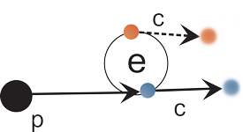
However, there is an apparent discrepancy between the theoretical prediction and the experimental data for the electron: experiments seem to indicate that the electron does not have any further constituents and that its size is several orders of magnitude smaller than the value given above. - This discrepancy vanishes if the experiments are examined from the perspective of the Basic Particle Model, for the following reasons. To investigate whether the electron is made up of constituent particles, it was bombarded with other particles (e.g. electrons or protons) at high energy. The electron did not break apart, so it was concluded that it does not have constituent parts. However, the Basic Particle Model states that the constituents of the electron do not have a mass on their own. So even if one of the constituent particles is accelerated by any arbitrary amount, the other constituent particle can follow. There is not even any force acting on that constituent. So an electron can never break up.
Figure 3.1: Experiment to break
up an electron
|
|||||||||||||||||||
|
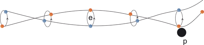
3.2 The Size of the Electron The investigation of the size of the electron is done by scattering an electron off a proton or another electron, for example, and investigating the angular distribution. If the Basic Particle Model is assumed for the electron, then only one of the constituents will be scattered. Such experiments are performed using highly relativistic electrons. Due to the time dilation the constituents of the electron will move along a considerably stretched helix. One of the constituents will pass the external particle as a normal, point-sized particle. The other constituent will only participate indirectly in this scattering process in that it causes the inertial behaviour of the overall configuration (i.e. the electron). The scattering will therefore be similar to that of a particle with a point-like size but with the mass of the electron. - From this result it is conventionally deduced that the electron is point-sized. |
|||||||||||||||||||
|
|
|||||||||||||||||||
|
From the above considerations it should be obvious that when the Basic Particle Model is applied to the electron, it does not contradict the experimental results. 4 Summary The "Basic Particle Model" provides a model for the understanding of the electron (as well as of other leptons and also of quarks), which is based on classical physics and agrees with experiment. And this model provides the cause of relativity on a 'mechanistic' basis. Also the refinement of the magnetic moment represented by the Landé factor can be explained classically. NOTE: The concept of the "Basic Particle Model" of matter was first presented at the Spring Conference of the German Physical Society (Deutsche Physikalische Gesellschaft) on 24 March 2000 in Dresden by Albrecht Giese. Comments are welcome to note@ag-physics.de. References: [1] Erwin Schrödinger, Über die kräftefreie Bewegung in der relativistischen Quantenmechanik ("On the free movement in relativistic quantum mechanics"), Berliner Ber., pp. 418-428 (1930). [2] J. Schwinger, On Quantum-Electrodynamics and the Magnetic Moment of the Electron, Phys.Rev.73, 416L (1948) 2021-05-16 |
|||||||||||||||||||
|
|
|||||||||||||||||||
|
Appendix A: The Mass of a Particle in General The mass equation in origin of mass was deduced on the assumption that the internal bond in an elementary particle is based only on the strong force. However, in order to understand the properties of the electron, the electric charge has to be taken into account too. Here we will briefly repeat the calculation using only the strong force, i.e. we will first calculate the mass of a particle without considering its electric charge. In order to follow the detailed derivation, please refer to origin of massIn the case of a pair of particles bound purely by the strong interaction, the Basic Particle Model indicates that the binding force is given by the following formula describing a multi-pole configuration: |
|||||||||||||||||||
|
|
(A.1) |
||||||||||||||||||
|
or for the absolute magnitude |
|||||||||||||||||||
|
|
(A.2) |
||||||||||||||||||
|
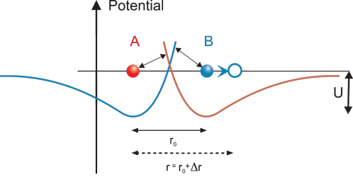
where F is the force caused by the field acting on the partner particle; S is the strength of the field which acts here to bind the two particles, belonging to the strong force; r is the distance between the two particles; and r0 the equilibrium distance (corresponding to Δr = 0) at which the force disappears. For the corresponding shape of the potential, refer to fig. A.1. | |||||||||||||||||||
|
Figure A.1: Potential of the bond between basic particles making up an elementary particle
|
|||||||||||||||||||
|
If we only consider small accelerations, where "small" means that during the time Δt (see below) the acceleration produces a change in velocity Δv << c, then we can for these changes replace the actual distance r in the denominator of eqs. (A.1) and (A.2) by the equilibrium distance r0 . If one particle (e.g. B) is now accelerated at a constant rate in the direction of the bond, then for a time |
|||||||||||||||||||
|
|
(A.3) |
||||||||||||||||||
|
after the start of the acceleration the other particle (A) will – due to the finite speed of light c - not receive any information about this change in position, and it will be held in its position by the original field. Then, after the initial period of Δt, particle A will also be accelerated constantly. From now, on the acceleration of particle A will follow the acceleration of particle B with this delay of Δt. This delay causes a constant displacement between the particles, which results in a constant force between them, given by (A.1). On the other hand, the current field of particle A will arrive at particle B after a further delay of Δt. Assuming a constant acceleration a, during this time 2Δt particle B will move a distance |
|||||||||||||||||||
|
|
(A.4) |
||||||||||||||||||
|
which is now added to the equilibrium distance. Due to this distance Δr1, the retarding force acting on particle B in the direction of motion, Fdm , will have the value |
|||||||||||||||||||
|
|
(A.5) |
||||||||||||||||||
|
and so, substituting for Δr1 from (A.4) |
|||||||||||||||||||
|
|
(A.6) |
||||||||||||||||||
|
Replacing Δt by r0 using the speed of light c (A.3) (i.e. with Δt = r0/c) yields |
|||||||||||||||||||
|
|
|
||||||||||||||||||
|
According to Newton’s definition, the quotient of F and a is the inertial mass m. So, |
|||||||||||||||||||
|
|
|
||||||||||||||||||
|
where Fdm is the force in the direction of the acceleration and mdm the corresponding inertial. And therefore: |
|||||||||||||||||||
|
|
|
||||||||||||||||||
|
Returning to eq. (A.5) we note that the full force |
|||||||||||||||||||
|
|
|
||||||||||||||||||
|
only acts if both the basic particles are positioned parallel to the direction of the applied force. We will now average the force over one circuit of the internal motion of the particle. This implies the assumption that the electron’s mass is measured using an acceleration perpendicular to the axis of the electron. The force changes in the course of the orbital motion and is given by |
|||||||||||||||||||
|
|
(A.7) |
||||||||||||||||||
|
where φ is the angle between (a) the direction of the binding force within the elementary particle and (b) the direction of acceleration. The average force is determined by integration: |
|||||||||||||||||||
|
|
(A.8) |
||||||||||||||||||
|
So the averaged, effective force is: |
|||||||||||||||||||
|
|
(A.9) |
||||||||||||||||||
|
Inserting Δr1 from eq. (A.4) now yields |
|||||||||||||||||||
|
|
(A.10) |
||||||||||||||||||
| and with the time delay Δt = r0/c: | (A.11) | ||||||||||||||||||
|
|
(A.12) |
||||||||||||||||||
|
and therefore: | |||||||||||||||||||
|
|
(A.13) |
||||||||||||||||||
|
or, in terms of the radius R = r0/2 of the electron: |
|||||||||||||||||||
 |
(A.14) |
||||||||||||||||||
|
We now determine S; (A.14) can be arranged as: |
|||||||||||||||||||
|
|
|
||||||||||||||||||
|
With the well known |
|||||||||||||||||||
| E = mc2 ... (also derived in Origin of Mass) this gives |
|
||||||||||||||||||
|
|
(A.15) |
||||||||||||||||||
|
Further we use: |
|||||||||||||||||||
|
|
|
||||||||||||||||||
|
from the assumption that the orbital frequency is the de Broglie frequency. From the geometry of the circular motion we have |
|||||||||||||||||||
|
|
|
||||||||||||||||||
|
from which it follows that |
|||||||||||||||||||
|
|
|
||||||||||||||||||
|
Substituting this in eq (A.15): |
|||||||||||||||||||
|
|
(A.16) |
||||||||||||||||||
|
Appendix B: The Landé factor We shall now determine the influence of the electric charge, particularly its influence on the magnetic moment of the electron. Without electric charge, only considering the strong interaction, the binding force is given by eq. (A.1): |
|||||||||||||||||||
|
|
|
||||||||||||||||||
|
where r0 is again the equivalence distance for F = 0. Now assuming two electric charges, e0/2 for each basic particle, the binding forces changes to: |
|||||||||||||||||||
|
|
(B.1) |
||||||||||||||||||
|
|
(B.2) |
||||||||||||||||||
| The electric charge causes a different equilibrium distance r = rz, for which the following must apply: | |||||||||||||||||||
|
|
(B.3) |
||||||||||||||||||
|
So it follows that for the new equilibrium distance: |
|||||||||||||||||||
|
|
(B.4) |
||||||||||||||||||
|
|
(B.5) |
||||||||||||||||||
|
To abbreviate this, we define |
|||||||||||||||||||
|
|
(B.6) |
||||||||||||||||||
|
from which it follows that: |
|||||||||||||||||||
|
|
(B.7) |
||||||||||||||||||
|
We can now write eq. (B.2) as |
|||||||||||||||||||
|
|
|
||||||||||||||||||
|
|
|
||||||||||||||||||
|
or with relation to rz, using eq. (B.7) |
|||||||||||||||||||
|
|
|
||||||||||||||||||
|
|
(B.8) |
||||||||||||||||||
|
Next we will determine ζ. By definition: |
|||||||||||||||||||
|
|
|
||||||||||||||||||
|
and we have (A.15) |
|||||||||||||||||||
|
|
|
||||||||||||||||||
|
and so |
|||||||||||||||||||
|
|
(B.9) |
||||||||||||||||||
|
We can now abbreviate this by using the definition of the fine structure constant: |
|||||||||||||||||||
|
|
(B.10) |
||||||||||||||||||
|
So we get |
|||||||||||||||||||
|
|
(B.11) |
||||||||||||||||||
|
Remembering that according to eq. (B.7) the classical equation for the magnetic moment of a charge orbiting at a velocity c and at a radius of R is given by: |
|||||||||||||||||||
|
|
(B.12) |
||||||||||||||||||
|
we will now have to replace the initially determined radius R by the corrected Rel (for the new equilibrium distance) to take into account the influence of the electric field: |
|||||||||||||||||||
|
|
(B.13) |
||||||||||||||||||
|
This replacement gives us a corrected magnetic moment of |
|||||||||||||||||||
|
|
(B.14) |
||||||||||||||||||
|
or, in terms to the Bohr magneton |
|||||||||||||||||||
|
|
|
||||||||||||||||||
|
(referring to (2.4) and (2.5)) we get |
|||||||||||||||||||
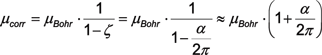 |
(B.15) |
||||||||||||||||||
|
the latter being the Julian Schwinger’s result (1948). – The correction factor in (B.15) has a numerical value of |
|||||||||||||||||||
|
|
(B.16) |
||||||||||||||||||
|
So the deviation of Schwinger's result from our result is approx. 10-6. - It should be noted that the original result of J. Schwinger deviates from the measured value also by approx. 10-6.
Conclusion: The Basic Particle Model is able to explain the Landé factor in a similar way to the new theoretical approach presented by J. Schwinger (a result for which he received the Nobel price in 1965). |
|||||||||||||||||||
|
|
|||||||||||||||||||